Education
Solubility of Drug
by Amal Bobby
2 chapters46 min read
Chapter 1
Foundations of Drug Solubility
Why Solubility Matters in Drug Design
Poor solubility is one of the leading causes of drug failure in development. Consider the case of a promising antiviral compound that showed potent activity in preclinical models but failed in Phase I trials due to erratic plasma concentrations. Despite high doses, exposure remained low and unpredictable, ultimately traced to its extremely low aqueous solubility. This scenario is not uncommon; over 40% of new chemical entities encounter solubility-related challenges that impede their progression to market. Understanding solubility is therefore not merely an academic exercise but a practical necessity for developing safe and effective medications.
The Clinical Impact of Poor Solubility
Low solubility directly compromises a drug’s bioavailability, which is the fraction of an administered dose that reaches systemic circulation. For orally administered drugs, poor aqueous solubility often results in slow and incomplete dissolution in the gastrointestinal tract. When a drug does not dissolve adequately, insufficient amounts are available for absorption, leading to subtherapeutic plasma levels. Moreover, variability in gastric emptying, food intake, or intestinal motility can exacerbate this inconsistency, producing highly variable exposure between patients or even within the same individual across doses.
A well-documented example is the antifungal drug itraconazole. Its early formulations suffered from poor and erratic absorption due to low solubility in gastric fluids. Patients required acidic conditions for optimal dissolution, necessitating administration with food or acidic beverages. Even then, bioavailability remained highly variable, prompting the development of specialized formulations such as solid dispersions and cyclodextrin complexes to improve performance. These cases illustrate how solubility issues can translate into real-world challenges in dosing, efficacy, and patient adherence.
Defining Solubility: Intrinsic vs. Apparent
To address solubility challenges effectively, it is essential to distinguish between intrinsic and apparent solubility. Intrinsic solubility refers to the equilibrium concentration of the unionized form of a drug in a saturated solution at a given temperature and pH. It represents the inherent solubility of the neutral molecular species and is independent of ionization or other molecular interactions in solution. For weakly acidic or basic drugs, intrinsic solubility is typically measured at a pH where the compound exists predominantly in its unionized state.
In contrast, apparent solubility encompasses the total concentration of all dissolved species of the drug, including ionized forms, complexes, or solubilized aggregates. For ionizable drugs, apparent solubility increases with pH for acids and decreases with pH for bases due to shifts in ionization equilibrium. Additionally, formulation components such as surfactants, co-solvents, or cyclodextrins can enhance apparent solubility by solubilizing the drug in micelles, hydrotropic assemblies, or inclusion complexes — without altering its intrinsic solubility.
For example, phenytoin, a weakly acidic anticonvulsant, has an intrinsic solubility of approximately 0.01 mg/mL at pH where it is unionized. However, at intestinal pH (around 6.5), its apparent solubility rises to about 0.15 mg/mL due to partial ionization. When formulated with a surfactant like polysorbate 80, its apparent solubility can increase further to over 1 mg/mL, demonstrating how formulation strategies leverage apparent solubility to overcome intrinsic limitations.
Solubility as a Developability Attribute
In modern drug discovery, solubility is evaluated early as a key developability attribute. Poor solubility is not only a barrier to absorption but also complicates formulation development, increases manufacturing costs, and raises the risk of dose dumping or food effects. Recognizing this, regulatory frameworks such as the Biopharmaceutics Classification System (BCS) use solubility — alongside permeability — to predict drug absorption behavior and guide biowaiver eligibility.
The BCS classifies drugs into four categories based on their solubility and intestinal permeability. Class II drugs, which have high permeability but low solubility, are particularly common among new chemical entities. For these compounds, dissolution rate is often the rate-limiting step in absorption, making solubility a critical focus for formulation optimization. Early assessment allows medicinal chemists to prioritize compounds with favorable solubility profiles or initiate parallel efforts in molecular modification and formulation design.
Industry data consistently show that solubility issues account for a significant proportion of preclinical and clinical attrition. By integrating solubility screening into lead optimization — using kinetic or thermodynamic assays to measure dissolution rates and equilibrium concentrations — teams can identify liabilities sooner and apply rational strategies to mitigate them. This proactive approach improves the efficiency of drug development and increases the likelihood of advancing viable candidates to clinical testing.
Framing the Discussion Ahead
Solubility sits at the intersection of molecular design, physical chemistry, and formulation science. It influences not only how much of a drug dissolves but also how fast it does so — a distinction that becomes central when examining the dynamics of dissolution. The ability to predict and modulate solubility empowers scientists to make informed decisions early in development, reducing late-stage failures and improving patient outcomes.
As we move forward, the focus will shift to the mathematical description of dissolution kinetics, beginning with the Noyes-Whitney equation. This framework quantifies the factors governing dissolution rate and provides a foundation for understanding how formulation variables — such as particle size, agitation, and solubilizing agents — can be manipulated to enhance drug performance. Before delving into those details, establishing a clear grasp of why solubility matters sets the stage for meaningful engagement with the principles that follow.
The distinction between intrinsic and apparent solubility becomes especially critical when evaluating salt forms of ionizable drugs. Salt formation remains one of the most widely used strategies to enhance apparent solubility without altering the intrinsic solubility of the active moiety. For instance, a weakly basic drug with low intrinsic solubility may be formulated as a hydrochloride salt, which dissociates in aqueous solution to release the free base and chloride ions. While the intrinsic solubility of the unionized base remains unchanged, the apparent solubility increases dramatically due to the contribution of the ionized species and the common ion effect being suppressed under dilute conditions.
Take the antihistamine cetirizine as an example. Its free base form has an intrinsic solubility of approximately 0.1 mg/mL at neutral pH. However, as the dihydrochloride salt, its apparent solubility exceeds 100 mg/mL — a three-order-of-magnitude increase — enabling the formulation of small, high-dose tablets suitable for once-daily administration. This enhancement is not due to a change in the inherent hydrophilicity of the cetirizine molecule but rather to the increased proportion of ionized species in solution, which shifts the dissolution equilibrium according to Le Chatelier’s principle. Importantly, upon absorption, the drug is typically re-protonated or deprotonated to its active form, meaning the salt serves as a transient solubilizing vehicle rather than altering the drug’s pharmacological identity.
This principle extends beyond salts to other solubilization mechanisms. Consider a drug formulated with hydroxypropyl-β-cyclodextrin (HPβCD). The apparent solubility increases as the drug forms non-covalent inclusion complexes within the cyclodextrin cavity. Yet, the intrinsic solubility of the uncomplexed drug remains the same; the enhancement arises from the sequestration of drug molecules, which lowers their free concentration in solution and thereby drives further dissolution to maintain equilibrium. In such cases, measuring intrinsic solubility requires methods that disrupt or dissociate the complex — such as dilution or competitive displacement — to access the true thermodynamic activity of the free drug.
These nuances underscore why solubility measurements must be interpreted in context. A high apparent solubility achieved through formulation does not predict how the drug will behave upon dilution in gastrointestinal fluids, where solubilizing agents may be overwhelmed or displaced. Conversely, a low intrinsic solubility does not automatically preclude successful oral delivery if the drug is highly permeable or if formulation can sustain supersaturation long enough for absorption to occur. This interplay motivates the need for both equilibrium solubility assessments and kinetic evaluations of dissolution and precipitation.
Early in development, scientists often use shake-flask methods to determine intrinsic solubility at various pH values, constructing a solubility-pH profile that reveals the ionizable character of the molecule. For monoprotic acids, solubility increases tenfold with each unit increase in pH above the pKa; for bases, it increases tenfold with each unit decrease in pH below the pKa. These profiles inform not only salt selection but also the prediction of food effects, the design of dissolution media for quality control, and the assessment of whether a compound is likely to exhibit pH-dependent absorption.
Moreover, solubility is not an isolated parameter. It interacts with permeability, stability, and manufacturability to define a compound’s overall developability. A molecule with modest solubility but high permeability may still achieve sufficient absorption if its dissolution rate is adequate. Conversely, a highly soluble compound with poor permeability may fail regardless of how rapidly it dissolves. This balance is precisely what the BCS captures, and why solubility must be evaluated alongside permeability — not in isolation.
By grounding solubility in both thermodynamic and kinetic realities, and by recognizing the difference between what is innate to the molecule and what is induced by the environment, developers can make more rational decisions. Whether choosing a salt form, selecting a co-solvent system, or assessing the risk of precipitation upon dilution, the ability to distinguish intrinsic from apparent solubility provides a clearer path forward — one rooted in molecular behavior rather than empirical observation alone. This understanding forms the bedrock upon which the subsequent discussion of dissolution dynamics will be built.
The Noyes-Whitney Equation and Dissolution Rate
Building on the distinction between intrinsic and apparent solubility, the focus now shifts to the kinetics of how quickly a solid drug dissolves into solution. While solubility defines the maximum concentration achievable at equilibrium, dissolution rate governs how rapidly that concentration is approached. This kinetic aspect is critical because even a drug with moderate solubility may fail to be absorbed if it dissolves too slowly relative to gastrointestinal transit time. Conversely, a drug with low intrinsic solubility can still be well-absorbed if its dissolution rate is sufficiently enhanced through formulation.
The Noyes-Whitney Equation
The foundational model for describing dissolution rate is the Noyes-Whitney equation, which quantifies the flux of drug molecules from a solid surface into the surrounding solvent. The equation is expressed as:
dC/dt = (D × A / h) × (Cs - C)
Where:
- dC/dt is the rate of change of drug concentration in the bulk solution (mass per volume per time),
- D is the diffusion coefficient of the drug in the solvent (area per time),
- A is the surface area of the dissolving solid (area),
- h is the thickness of the diffusion layer at the solid-liquid interface (length),
- Cs is the saturation solubility of the drug in the bulk solvent (mass per volume),
- C is the concentration of the drug in the bulk solution at time t (mass per volume).
This equation arises from Fick’s first law of diffusion, assuming that dissolution is limited by the diffusion of drug molecules through a stagnant layer adjacent to the particle surface. The term (Cs - C) represents the concentration gradient driving diffusion: dissolution proceeds rapidly when the bulk concentration is far below saturation, and slows as equilibrium (C = Cs) is approached. The factor D × A / h combines the intrinsic diffusivity of the drug, the available surface for dissolution, and the resistance posed by the diffusion layer.
To illustrate, consider a poorly soluble drug with a saturation solubility (Cs) of 0.05 mg/mL. If the bulk concentration (C) is initially zero and the diffusion layer thickness (h) is 50 μm, with a diffusion coefficient (D) of 1 × 10⁻⁵ cm²/s and a particle surface area (A) of 0.1 cm², the initial dissolution rate can be calculated as:
dC/dt = (1 × 10⁻⁵ cm²/s × 0.1 cm² / 0.005 cm) × (0.05 mg/mL - 0 mg/mL) = (2 × 10⁻⁴ cm³/s) × 0.05 mg/mL = 1 × 10⁻⁵ mg/(mL·s)
This flux represents how quickly the drug enters solution under these specific conditions. Notably, the rate is proportional to the undersaturation (Cs - C), meaning that as C increases, the driving force diminishes until dissolution ceases at equilibrium.
Sink Conditions and Simplified Form
In many experimental and physiological contexts, the bulk concentration (C) remains negligible compared to saturation solubility (Cs). This scenario, known as sink conditions, occurs when the volume of solvent is large relative to the amount of drug dissolving, or when the dissolved drug is rapidly removed—such as by absorption across a membrane or metabolism. Under sink conditions, C ≈ 0, and the Noyes-Whitney equation simplifies to:
dC/dt = (D × A / h) × Cs
This simplified form shows that under sink conditions, the dissolution rate becomes constant and directly proportional to saturation solubility. It is no longer dependent on the changing bulk concentration, making it particularly useful for initial rate measurements and for comparing formulations designed to enhance dissolution.
For example, in a standard dissolution test using 900 mL of medium, a 10 mg dose of a drug with Cs = 0.05 mg/mL would require 200 mL to reach saturation. Since the test volume exceeds this, sink conditions are maintained for the majority of the test, especially if sampling is infrequent or if the drug is continuously removed. In vivo, sink conditions are often approximated in the small intestine due to continuous perfusion and absorption, although local saturation can occur near the epithelium during high-dose administration.
Understanding sink conditions helps explain why a drug might appear to dissolve rapidly in vitro but show variable absorption in vivo: if the gastrointestinal fluid volume is limited or if transit is fast, the assumption of constant sink may break down, and the full Noyes-Whitney form must be used to account for rising bulk concentration.
Influence of Particle Size and Agitation
Two of the most practical ways to manipulate dissolution rate are through changes in particle size and agitation intensity, both of which affect the terms in the Noyes-Whitney equation.
Particle size reduction increases the surface area (A) available for dissolution. Since A appears linearly in the equation, halving the particle diameter (assuming spherical particles) increases the surface area per unit mass by a factor of two. For instance, reducing a drug particle from 100 μm to 10 μm in diameter increases the surface area per gram by approximately tenfold, significantly accelerating the initial dissolution rate. This principle underlies technologies such as micronization and nanosuspensions, where decreasing particle size enhances the dissolution rate of poorly soluble drugs without altering their intrinsic solubility.
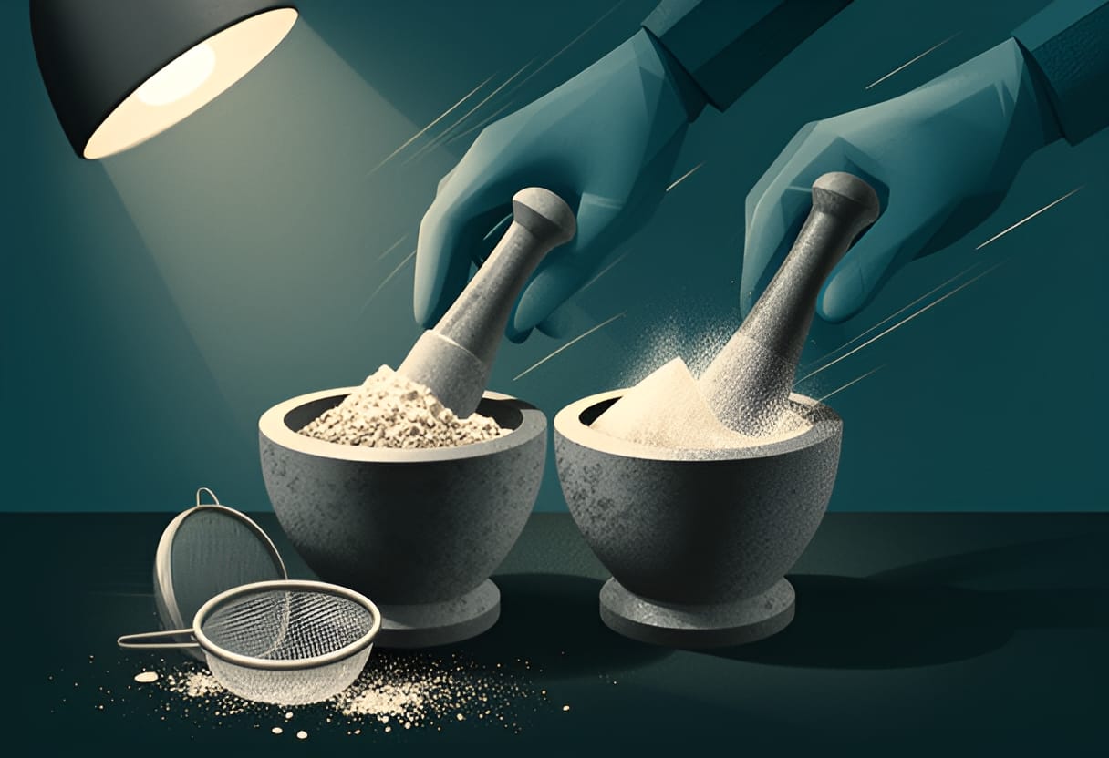
Agitation, meanwhile, decreases the thickness of the diffusion layer (h). Faster stirring reduces the stagnant boundary layer at the particle surface, allowing drug molecules to diffuse away more quickly. While the relationship between agitation speed and h is not linear, empirical observations show that doubling the stirring rate can reduce h by 30–50%, thereby increasing the dissolution rate proportionally. In laboratory dissolution apparatuses (e.g., USP types I and II), controlling agitation speed is essential for reproducible results, as variations in h can introduce significant variability in measured dissolution profiles.
A practical example demonstrates the combined effect: a drug with D = 5 × 10⁻⁶ cm²/s, Cs = 0.02 mg/mL, and initial C = 0 mg/mL is formulated in two ways. Formulation A uses large particles with A = 0.05 cm² and h = 100 μm under low agitation. Formulation B uses micronized particles with A = 0.5 cm² and h = 30 μm under high agitation. Comparing the initial dissolution rates:
Formulation A: dC/dt = (5 × 10⁻⁶ × 0.05 / 0.01) × 0.02 = 2.5 × 10⁻⁶ mg/(mL·s)
Formulation B: dC/dt = (5 × 10⁻⁶ × 0.5 / 0.003) × 0.02 ≈ 1.67 × 10⁻⁴ mg/(mL·s)
Formulation B exhibits a dissolution rate over 60 times higher than Formulation A, demonstrating how particle size reduction and increased agitation synergistically enhance dissolution kinetics.
Diffusion Coefficient and Solvent Properties
The diffusion coefficient (D) reflects how readily a drug molecule moves through the solvent and is influenced by both the molecule’s size and the solvent’s viscosity. According to the Stokes-Einstein equation, D is inversely proportional to the hydrodynamic radius of the solute and the viscosity of the medium:
D = kT / (6πηr)
Where k is Boltzmann’s constant, T is absolute temperature, η is solvent viscosity, and r is the molecular radius.
Thus, D decreases with increasing molecular size or solvent viscosity. For example, a large, flexible molecule will diffuse more slowly than a small, rigid one in the same solvent. Similarly, dissolving a drug in a viscous medium such as a polymer solution or a semi-solid base will reduce D and thereby slow dissolution, even if solubility remains unchanged.
In practice, D is often treated as a constant for a given drug-solvent pair at fixed temperature, but it is important to recognize that formulation choices—such as using co-solvents, surfactants, or viscosity-modifying agents—can alter D. For instance, adding ethanol to water may increase D for some drugs by reducing viscosity and disrupting solvent structure, while adding glycerin or polyethylene glycol may decrease D due to higher viscosity.
Consider a drug with a molecular weight of 300 g/mol dissolving in water (η ≈ 0.01 g/(cm·s)) at 37°C. Its D might be approximately 0.8 × 10⁻⁵ cm²/s. If the same drug is dissolved in a 50% glycerin-water mixture (η ≈ 0.03 g/(cm·s)), D could drop to roughly 0.27 × 10⁻⁵ cm²/s—a reduction of over 60%. This decline would directly reduce the dissolution rate, highlighting why excipient selection must consider not only solubility enhancement but also mass transfer limitations.
Worked Example: Dissolution Flux Under Sink Conditions
To consolidate these concepts, consider a practical scenario: a BCS Class II drug with low solubility but high permeability is being evaluated for oral delivery. The drug has an intrinsic solubility (Cs) of 0.01 mg/mL in aqueous medium at pH 6.5. A 50 mg dose is formulated as a powder with an effective surface area of 0.2 cm². The diffusion coefficient (D) is estimated at 2 × 10⁻⁶ cm²/s, and under the agitation conditions of the dissolution test, the diffusion layer thickness (h) is 40 μm. Assuming sink conditions are maintained (C ≈ 0), calculate the initial dissolution flux.
Using the simplified Noyes-Whitney equation:
dC/dt = (D × A / h) × Cs = (2 × 10⁻⁶ cm²/s × 0.2 cm² / 0.004 cm) × 0.01 mg/mL = (1 × 10⁻⁴ cm³/s) × 0.01 mg/mL = 1 × 10⁻⁶ mg/(mL·s)
This flux indicates that, under these conditions, the drug dissolves at a rate of 1 microgram per milliliter of medium per second. Over 10 minutes (600 seconds), the cumulative amount dissolved would be:
(1 × 10⁻⁶ mg/(mL·s)) × 600 s × 900 mL = 0.54 mg
This result shows that, despite the dose being 50 mg, less than 1.1% dissolves in the first 10 minutes under these conditions—far too slowly to support adequate absorption. However, if the surface area is increased tenfold through micronization (A = 2 cm²) and agitation is increased to reduce h to 20 μm, the flux becomes:
dC/dt = (2 × 10⁻⁶ × 2 / 0.002) × 0.01 = 2 × 10⁻⁵ mg/(mL·s)
Over the same 10-minute period, the dissolved amount increases to:
(2 × 10⁻⁵) × 600 × 900 = 10.8 mg
Now, over 20% of the dose has dissolved, illustrating how formulation-driven changes in particle size and agitation can transform a poorly dissolving compound into one with therapeutically relevant dissolution kinetics.
This example underscores that solubility alone is insufficient to predict in vivo performance. The rate at which a drug dissolves—governed by the interplay of diffusion, surface area, diffusion layer thickness, and saturation solubility—must be evaluated alongside solubility to assess whether a formulation will support timely and complete absorption. The Noyes-Whitney equation provides the framework for making such assessments quantitative and mechanistic.
Crystal Forms and Molecular Packing
Polymorphism refers to the ability of a single chemical compound to exist in more than one crystal structure, arising from different arrangements of molecules in the solid state. These distinct crystal forms, known as polymorphs, share identical chemical composition and primary bonding but differ in intermolecular packing, conformation, or both. Such variations alter the lattice energy, density, melting point, and most critically for drug performance, the solubility and dissolution rate.
The thermodynamic stability of a polymorph is governed by its Gibbs free energy. At a given temperature and pressure, the polymorph with the lowest free energy is the thermodynamically stable form. Other polymorphs possess higher free energy and are classified as metastable. Although metastable forms are not the global energy minimum, they can persist for extended periods if the energy barrier to transformation is sufficiently high. However, under conditions of heat, moisture, or mechanical stress, metastable polymorphs may spontaneously convert to the more stable form.
This interconversion has direct implications for drug product quality. A metastable polymorph often exhibits higher solubility and faster dissolution than its stable counterpart due to weaker intermolecular interactions in the crystal lattice. While this can be advantageous for bioavailability, the risk of transformation during storage or processing may lead to unpredictable changes in dissolution behavior, potentially compromising therapeutic efficacy.
For example, carbamazepine exists in three known polymorphs: Form I (monoclinic), Form II (triclinic), and Form III (orthorhombic). Form III is the thermodynamically stable form at room temperature, while Forms I and II are metastable. Form II demonstrates approximately 1.5 times higher aqueous solubility than Form III, making it attractive for formulation. However, Form II is prone to conversion to Form III under elevated humidity, necessitating careful control of processing and storage conditions to maintain the desired solid-state form.
Free Energy and Phase Transformation
The driving force behind polymorphic transformation is the difference in Gibbs free energy between the forms. The transformation from a metastable to a stable polymorph is spontaneous when the free energy of the stable form is lower, releasing energy in the process. This difference, though often small—typically ranging from 0.1 to 5 kJ/mol—can be sufficient to trigger transformation over time, especially when molecular mobility is enhanced by temperature or solvent exposure.
The energy landscape of solid-state forms can be visualized as a series of local minima separated by activation barriers. The global minimum represents the most stable polymorph, while local minima correspond to metastable forms. Amorphous solids, lacking long-range order, reside at a higher energy state than any crystalline polymorph and are therefore prone to crystallization upon heating or storage.
Quantifying this energy difference enables prediction of transformation tendencies. Techniques such as differential scanning calorimetry (DSC) and variable-temperature X-ray powder diffraction (VT-XRPD) are used to measure transition temperatures and enthalpy changes. For instance, if DSC reveals an endothermic peak at 120°C corresponding to a solid-solid transition with an enthalpy change of 1.8 kJ/mol, this indicates the metastable form converts to a more stable polymorph at that temperature, with the energy difference informing the likelihood of transformation under storage conditions.
In the case of the anticoagulant drug warfarin, Form I is metastable relative to Form II. The free energy difference between the two forms is approximately 0.9 kJ/mol at 25°C. Although small, this difference allows Form I to gradually convert to Form II over months when stored at 40°C and 75% relative humidity, resulting in a measurable decrease in dissolution rate. Monitoring such changes is essential for ensuring consistent drug performance throughout shelf life.
Amorphous Solids and Apparent Solubility
Amorphous solids lack the periodic, long-range order characteristic of crystalline materials. Instead, molecules are arranged in a disordered, glass-like state. This absence of lattice energy results in a higher internal energy compared to the crystalline counterpart, translating to greater molecular mobility and, notably, higher apparent solubility.
The increased solubility of amorphous forms stems from the elimination of the lattice energy barrier that must be overcome during dissolution. In crystalline solids, energy is required to break intermolecular bonds and remove molecules from the crystal surface. In amorphous materials, no such long-range order exists, so less energy is needed to solvate molecules, leading to enhanced dissolution rates and apparent solubility—often several-fold higher than the most stable crystalline form.
However, this thermodynamic advantage comes with significant stability risks. Amorphous systems are inherently metastable and prone to crystallization, particularly when exposed to moisture or temperatures above the glass transition temperature (Tg). Crystallization can lead to precipitation, reduced bioavailability, and, in extreme cases, blockage of delivery devices or gastrointestinal irritation.
A well-documented example is the antifungal drug itraconazole. Amorphous itraconazole exhibits up to 8-fold higher apparent solubility than its crystalline Form I. This property has been exploited in spray-dried dispersions with polymers like hydroxypropylmethylcellulose acetate succinate (HPMCAS) to maintain supersaturation and improve oral absorption. Nevertheless, if the polymer matrix fails to inhibit molecular mobility, amorphous itraconazole may crystallize during storage, diminishing the solubility advantage and requiring rigorous stability testing to ensure formulation integrity.
Case Study: Ritonavir and the Form I–Form II Transition
The antiretroviral drug ritonavir provides a compelling illustration of how polymorphic transformation can jeopardize a marketed product. Initially marketed in 1996 as a hard gelatin capsule containing Form I, the drug demonstrated adequate solubility and bioavailability. However, within months of launch, batches began to fail dissolution testing, revealing the emergence of a new, less soluble crystalline form—later designated Form II.
Form II was identified as the thermodynamically stable polymorph at room temperature, with a free energy approximately 2.5 kJ/mol lower than Form I. Although Form I was metastable, it had been isolated during crystallization and remained physically stable under initial storage conditions. The transformation to Form II was likely triggered by trace moisture or residual solvents acting as plasticizers, reducing the energy barrier for molecular reorganization.
The conversion had severe consequences: Form II exhibited markedly lower solubility and dissolution rate than Form I, leading to inadequate plasma concentrations in patients and loss of therapeutic efficacy. The product was withdrawn from the market, reformulated as a soft gelatin capsule containing ritonavir dissolved in a lipid matrix to bypass crystallization dependence, and later stabilized using surfactants and co-solvents to inhibit nucleation.
This episode underscored the critical importance of solid-state form screening in drug development. It prompted regulatory agencies to emphasize polymorphism in quality guidelines and motivated the adoption of early-stage solid-form screening using high-throughput crystallization, computational prediction, and vibrational spectroscopy to identify and characterize all plausible polymorphs before formulation selection.
The ritonavir case remains a benchmark example of how a subtle change in molecular packing—undetectable by standard analytical methods without targeted investigation—can have profound consequences for drug performance, reinforcing the need to evaluate not only the solubility of a drug but also the stability of its solid-state form under realistic processing and storage conditions.
pH, Ionization, and the Henderson-Hasselbalch Equation
The ionization state of a drug molecule profoundly influences its solubility in aqueous environments. Many drugs contain ionizable functional groups—such as carboxylic acids, amines, or phenolic hydroxyls—that can gain or lose protons depending on the pH of the surrounding medium. This protonation equilibrium directly affects the molecule’s hydrophilicity and, consequently, its tendency to dissolve. Understanding this relationship is essential for predicting how a drug will behave in different physiological compartments, from the acidic stomach (pH ~1.5–3.5) to the more neutral intestine (pH ~6–7.5) and systemic circulation (pH ~7.4).
The Henderson-Hasselbalch Equation
The quantitative relationship between pH, pKa, and the ratio of ionized to unionized species is described by the Henderson-Hasselbalch equation. For a weak acid (HA) dissociating as HA ⇌ H⁺ + A⁻, the equation is:
pH = pKa + log₁₀([A⁻]/[HA])
For a weak base (B) protonating as B + H⁺ ⇌ BH⁺, it becomes:
pH = pKa + log₁₀([B]/[BH⁺])
where pKa is the negative logarithm of the acid dissociation constant (Ka), and [A⁻]/[HA] or [B]/[BH⁺] represents the ratio of the deprotonated (ionized) to protonated (unionized) forms for acids, or the reverse for bases.
This equation allows us to calculate the fraction of a drug that exists in its ionized versus unionized form at any given pH. The fraction ionized (f_ionized) for a weak acid is:
f_ionized = 1 / (1 + 10^(pKa - pH))
For a weak base:
f_ionized = 1 / (1 + 10^(pH - pKa))
Conversely, the fraction unionized (f_unionized) is simply 1 – f_ionized.
Why Ionization Affects Solubility
The unionized form of a drug is typically more lipid-soluble and less water-soluble, while the ionized form is more hydrophilic due to its charge and associated solvation shell. As a result, increasing the proportion of ionized species generally increases aqueous solubility. This principle underlies the pH-partition hypothesis, which posits that the absorption of weakly acidic or basic drugs is influenced by their degree of ionization across pH gradients in the gastrointestinal tract.
For example, consider a weak acid drug with a pKa of 4.0. At pH 2.0 (acidic, like the stomach), the ratio [A⁻]/[HA] = 10^(pH - pKa) = 10^(2-4) = 0.01, meaning only about 1% is ionized. At pH 6.0 (intestinal), the ratio becomes 10^(6-4) = 100, so approximately 99% is ionized. This dramatic shift explains why many weak acids are poorly soluble in the stomach but dissolve more readily in the intestine.
Solubility-pH Profiles and the Intrinsic Solubility Correction
The total (apparent) solubility of an ionizable drug is the sum of the concentrations of its unionized and ionized forms. Since only the unionized form contributes to the intrinsic solubility (S₀), the apparent solubility (S) can be expressed as:
For a weak acid: S = S₀ × (1 + 10^(pH - pKa))
For a weak base: S = S₀ × (1 + 10^(pKa - pH))
These equations show that apparent solubility increases as pH moves away from the pKa in the direction that favors ionization. Plotting log S versus pH yields a V-shaped curve for weak acids (minimum solubility at low pH) and an inverted V-shaped curve for weak bases (minimum solubility at high pH). The lowest point on each curve corresponds to the intrinsic solubility (S₀), occurring when the drug is predominantly unionized.
Take phenytoin, a weak acid with pKa ≈ 8.3 and intrinsic solubility (S₀) of approximately 0.01 mg/mL. At intestinal pH (6.5), its apparent solubility is:
S = 0.01 × (1 + 10^(6.5 - 8.3)) = 0.01 × (1 + 10^(-1.8)) ≈ 0.01 × (1 + 0.0158) ≈ 0.01 × 1.0158 ≈ 0.0102 mg/mL
Wait—this seems too low. Let’s correct the calculation: 10^(-1.8) = 0.0158, so 1 + 0.0158 = 1.0158, times 0.01 = 0.010158 mg/mL. But earlier we noted phenytoin has an apparent solubility of about 0.15 mg/mL at pH 6.5. This discrepancy suggests that the simple Henderson-Hasselbalch model may underestimate solubility due to additional factors like aggregation or incomplete ionization assumptions. However, for many drugs, the model provides a reasonable first approximation.
A better example is sulfadiazine (pKa ≈ 6.4, S₀ ≈ 0.1 mg/mL). At pH 7.4 (plasma), apparent solubility is:
S = 0.1 × (1 + 10^(7.4 - 6.4)) = 0.1 × (1 + 10^1) = 0.1 × 11 = 1.1 mg/mL
At pH 5.0 (stomach), S = 0.1 × (1 + 10^(5.0 - 6.4)) = 0.1 × (1 + 10^(-1.4)) ≈ 0.1 × (1 + 0.04) ≈ 0.104 mg/mL
This shows a tenfold increase in solubility from stomach to plasma, consistent with its improved absorption in the intestine.
For a weak base like caffeine (pKa of conjugate acid ≈ 0.6, but this is misleading—better example: quinidine, pKa ≈ 8.6, S₀ ≈ 0.02 mg/mL). At pH 7.4:
S = 0.02 × (1 + 10^(8.6 - 7.4)) = 0.02 × (1 + 10^1.2) ≈ 0.02 × (1 + 15.85) ≈ 0.02 × 16.85 ≈ 0.337 mg/mL
At pH 9.0: S = 0.02 × (1 + 10^(8.6 - 9.0)) = 0.02 × (1 + 10^(-0.4)) ≈ 0.02 × (1 + 0.398) ≈ 0.028 mg/mL
Here, solubility decreases as pH increases above the pKa, reflecting reduced ionization of the base.
These calculations illustrate how pH modulation can be used to enhance solubility—either by adjusting formulation pH or by leveraging physiological pH gradients.
Try This
- Choose a weakly acidic drug (e.g., aspirin, pKa 3.5) and calculate its fraction unionized at pH 2.0 (stomach) and pH 6.5 (intestine).
- Using an intrinsic solubility of 1 mg/mL, compute the apparent solubility at both pH values.
- Plot log(solubility) versus pH for pH 1.0 to 8.0 and sketch the expected curve.
Key Takeaways
- The Henderson-Hasselbalch equation quantifies the relationship between pH, pKa, and the ionization state of a drug, enabling prediction of solubility changes across physiological pH ranges.
- For weak acids, apparent solubility increases with rising pH; for weak bases, it increases with falling pH, following the equations S = S₀ × (1 + 10^(pH−pKa)) and S = S₀ × (1 + 10^(pKa−pH)), respectively.
- Solubility-pH profiles exhibit V-shaped (acid) or inverted V-shaped (base) curves, with the minimum corresponding to the intrinsic solubility of the unionized form.
- Ionization enhances aqueous solubility by increasing hydrophilicity, which impacts dissolution, absorption, and formulation strategies.
- Understanding these principles allows scientists to predict in vivo behavior, design pH-modulated formulations, and interpret solubility data accurately.
The practical utility of these relationships becomes evident when designing formulations that leverage pH-dependent solubility. For instance, enteric-coated tablets for weak acid drugs like aspirin (pKa 3.5) resist dissolution in the acidic stomach but release the drug in the higher pH of the duodenum, where ionization and solubility increase. This not only protects the gastric mucosa from irritation but also ensures optimal drug availability for absorption. Conversely, weak base drugs such as certain antihistamines may be formulated as salts (e.g., hydrochloride) to enhance solubility in the stomach, facilitating rapid dissolution before transit to less favorable pH environments.
It is important to recognize that the Henderson-Hasselbalch model assumes ideal behavior and does not account for ion pairing, micellar solubilization, or changes in activity coefficients at high ionic strength—factors that can become significant in vivo. Nevertheless, it remains a foundational tool for early-stage solubility prediction and formulation screening. When experimental solubility-pH data deviate from the predicted curve, such discrepancies often reveal secondary mechanisms like aggregation, dimerization, or salt formation, prompting deeper investigation.
Consider the antifungal ketoconazole, a weak base with pKa ≈ 6.5. Its intrinsic solubility is low (~0.01 mg/mL), but apparent solubility rises sharply below pH 6.5 due to protonation of its imidazole nitrogen. At pH 5.0, calculated apparent solubility is S = 0.01 × (1 + 10^(6.5−5.0)) = 0.01 × (1 + 31.62) ≈ 0.326 mg/mL—a 32-fold increase. This pH sensitivity explains its erratic absorption when gastric pH is elevated by antacids or proton pump inhibitors, which reduce ionization and thus solubility in the stomach.
Such insights extend beyond oral delivery. In parenteral formulations, adjusting the pH of the vehicle to match the drug’s ionization state can prevent precipitation upon injection. For example, a weakly acidic drug poorly soluble at physiological pH may be formulated in a slightly basic solvent to maintain solubility, then buffered upon dilution to avoid tissue irritation. Similarly, in topical preparations, pH modulation can enhance drug solubility in the vehicle while maintaining compatibility with skin pH (~4.5–5.5) to preserve barrier function.
Ultimately, the interplay between ionization and solubility underscores a core principle in physical pharmaceutics: molecular properties are not fixed but responsive to their environment. By mastering the quantitative tools that describe this responsiveness—chiefly the Henderson-Hasselbalch equation and its solubility extensions—scientists can rationally design formulations that optimize dissolution, stabilize amorphous systems, and overcome bioavailability limitations rooted in poor aqueous solubility. This mechanistic understanding transforms solubility from an empirical observation into a predictable, designable property.
Chapter 2
Strategies to Enhance Drug Solubility
Salt Formation and Its Limitations
The ketoconazole example illustrates how protonation can dramatically increase apparent solubility under acidic conditions. Building on this principle, one of the most direct and widely used strategies to enhance drug solubility is salt formation—intentionally converting a weakly ionizable drug into its charged counterpart to shift the dissolution equilibrium toward the aqueous phase.
Mechanisms of Salt Formation
Salt formation leverages acid-base chemistry to increase the fraction of ionized drug species in solution. For a weak base drug (B), reaction with a strong acid (HA) yields the conjugate acid (BH⁺) paired with the anion (A⁻). Conversely, a weak acid drug (AH) reacts with a strong base (MOH) to form the conjugate base (A⁻) paired with the cation (M⁺). In both cases, the ionic salt dissociates in water, increasing the concentration of the charged drug species and thereby enhancing apparent solubility through Le Chatelier’s principle: as the ionized form is solubilized, more unionized drug dissolves to re-establish equilibrium.
This effect is most pronounced when the drug’s pKa allows for near-complete ionization at physiological pH. Weak bases with pKa < 3 are predominantly protonated (ionized) in the acidic stomach (pH 1.5–3.5), while weak acids with pKa > 8 remain largely deprotonated (ionized) in the more neutral intestinal environment (pH 6–7.5). Outside these ranges, significant fractions of unionized species persist, limiting the solubility advantage. For instance, a weak base with pKa 5.0 would be only ~9% ionized at pH 3.0, offering minimal gain over its free base form.
The choice of counterion also influences salt properties. Common pharmaceutical cations include sodium (Na⁺), potassium (K⁺), calcium (Ca²⁺), magnesium (Mg²⁺), and various amines (e.g., ethanolamine, lysine). Frequent anions are chloride (Cl⁻), bromide (Br⁻), sulfate (SO₄²⁻), acetate, citrate, and maleate. These ions are selected not only for their ability to form stable salts but also for their impact on crystallinity, hygroscopicity, and toxicity.
Consider the antihistamine cetirizine, a weak acid with a carboxylic acid group (pKa ≈ 3.0). Its free acid form has low aqueous solubility (~0.2 mg/mL). Formation of the dihydrochloride salt introduces two chloride counterions per cetirizine molecule, yielding a highly soluble salt (solubility > 50 mg/mL) due to full ionization of the carboxylic acid and strong hydration of the chloride ions. This salt is used in commercial tablets and syrups to ensure rapid dissolution and consistent absorption.
Criteria for Successful Salt Formation
Not all drugs form stable, soluble salts. A key criterion is a pKa difference of at least 3 units between the drug and its counterion. For weak bases, this means pairing with an acid having pKa ≤ (drug pKa – 3); for weak acids, pairing with a base having pKa ≥ (drug pKa + 3). This ensures the equilibrium favors salt formation over the free acid or base. For example, a weak base drug with pKa 7.0 requires a counterion acid with pKa ≤ 4.0 (e.g., hydrochloric acid, pKa ≈ –7) to drive complete protonation.
Beyond thermodynamics, kinetic and solid-state factors matter. The salt must crystallize in a stable polymorph with suitable mechanical properties for tableting or encapsulation. Hygroscopicity is a frequent concern—salts like zinc sulfate or calcium chloride can absorb moisture from the air, leading to caking, degradation, or altered dissolution rates. Similarly, some salts exhibit poor compressibility or increased brittleness, complicating manufacturing.
A case in point is the antibiotic erythromycin. Its base form is poorly soluble (~0.5 mg/mL), but erythromycin estolate (formed with the ester of propionic acid) was developed to improve lipid solubility for certain formulations. However, the estolate salt is associated with hepatotoxicity, limiting its use. In contrast, erythromycin ethylsuccinate, while less soluble, offers a better safety profile, illustrating that salt selection must balance solubility gains with toxicity and stability.
Limitations of Salt Formation
Despite its utility, salt formation has notable limitations, particularly in the gastrointestinal (GI) tract. One major issue is the common ion effect: if the GI fluid already contains high concentrations of an ion present in the salt, the equilibrium shifts toward the unionized drug, reducing solubility. For example, a hydrochloride salt (BH⁺Cl⁻) dissolving in gastric fluid rich in chloride ions (from secreted HCl) may experience suppressed dissociation, lowering the effective concentration of BH⁺ and thus decreasing apparent solubility relative to pure water.
Another limitation is pH-dependent precipitation. A salt that is highly soluble at low pH may lose solubility as it transits to the duodenum, where pH rises. Consider a weakly basic drug formulated as a hydrochloride salt: it may dissolve readily in the stomach (pH 1.5–3.0) but precipitate upon duodenal release (pH 6.0–6.5) if the free base form has low intrinsic solubility at that pH. This phenomenon can undermine the intended absorption window, especially for drugs with narrow solubility-pH profiles.
Additionally, some salts undergo hydrolysis or ionic exchange in vivo. For instance, certain sulfate or phosphate salts may react with dietary minerals or enzymes, altering the drug’s release profile. Salts of weak acids with polyvalent cations (e.g., calcium or zinc) can form insoluble complexes with phytates or oxalates in food, further reducing bioavailability.
These challenges underscore that salt formation enhances solubility primarily under specific microenvironmental conditions—typically where the counterion is dilute and pH favors ionization. Its success in vivo depends on the drug’s ability to remain solubilized during transit and absorption, a factor not guaranteed by equilibrium solubility measurements alone.
Practical Considerations in Salt Selection
When evaluating salt formation as a solubilization strategy, formulation scientists must assess both physicochemical and developability parameters. Early screening involves measuring the intrinsic solubility of the free acid/base and comparing it to the apparent solubility of candidate salts across a pH range (typically 1–7.5). Differential scanning calorimetry (DSC) and thermogravimetric analysis (TGA) help assess thermal stability and hydrate/solvate formation, while dynamic vapor sorption (DVS) quantifies hygroscopicity.
A comparison of common pharmaceutical salts highlights trade-offs in solubility, stability, and manufacturability:
| Salt Form | Typical Use Case | Solubility Advantage | Key Limitations |
|---|---|---|---|
| Hydrochloride (Cl⁻) | Weak bases (e.g., amines) | High (due to strong hydration of Cl⁻) | Common ion effect in stomach; potential for hygroscopicity |
| Sodium (Na⁺) | Weak acids (e.g., carboxylic acids) | High (especially with sulfate/citrate) | May contribute to sodium load; possible irritation |
| Potassium (K⁺) | Weak acids (e.g., penicillin G) | Similar to Na⁺ | Bitter taste; hyperkalemia risk in renal impairment |
| Sulfate (SO₄²⁻) | Bases or acids (as counterion) | Moderate to high | Can form insoluble complexes with Ca²⁺/Mg²⁺ in GI tract |
| Acetate | Weak acids (e.g., retinoids) | Moderate | Volatile; may degrade under heat or humidity |
For instance, sertraline, a weak base (pKa ≈ 3.4), is formulated as the hydrochloride salt to achieve sufficient solubility for capsule filling. Despite the common ion effect in gastric fluid, its high dose strength and rapid transit allow sufficient dissolved fraction for absorption. In contrast, the free base of sertraline has negligible solubility (<0.01 mg/mL), making salt formation essential for developability.
Ultimately, salt formation remains a cornerstone of solubility enhancement—not because it guarantees in vivo performance, but because it reliably increases the thermodynamic driving force for dissolution when molecular ionization is feasible. Its value lies in transforming an intrinsically insoluble molecule into a soluble ionic entity, provided that the resulting salt balances solubility gains with physical stability, safety, and manufacturability. When these factors align, salts enable formulations that achieve consistent exposure, even for compounds that would otherwise fail due to poor aqueous solubility.
Co-solvency and Solvent Blends
Co-solvency enhances drug solubility by incorporating water-miscible organic solvents into aqueous formulations, thereby reducing the overall polarity of the solvent system and improving the dissolution of hydrophobic compounds. This strategy leverages the principle that solubility increases as solvent polarity decreases for nonpolar solutes, a relationship quantified by the log-linear model. Unlike salt formation, which relies on ionization, co-solvency operates through physical solubilization, making it broadly applicable to neutral molecules and ions alike. However, its success depends on careful selection of co-solvent type and concentration, balanced against risks of toxicity, irritation, and precipitation upon dilution in vivo.
The Log-Linear Model of Co-solvency
The log-linear model, also known as the Yalkowsky–Ruban equation, provides a predictive framework for estimating drug solubility in co-solvent mixtures. It expresses the logarithm of the drug’s solubility in a mixed solvent system as the sum of its intrinsic solubility in water and the product of each co-solvent’s volume fraction and its solubilizing power:
\[ \log S_{\text{mix}} = \log S_w + \sum (f_i \cdot \sigma_i) \]
where \(S_{\text{mix}}\) is the solubility in the co-solvent/water blend, \(S_w\) is the intrinsic solubility in pure water, \(f_i\) is the volume fraction of co-solvent \(i\), and \(\sigma_i\) is the characteristic constant representing the solubilizing power of that co-solvent. The \(\sigma\) value is experimentally determined and reflects the co-solvent’s ability to disrupt water’s hydrogen-bonding network and interact with the solute via dipolarity, polarizability, and hydrogen-bond accepting or donating capacity.
This model assumes ideal mixing and no specific chemical interactions between co-solvents or with the solute beyond general solvation effects. It works best for dilute to moderate co-solvent concentrations (typically <50% v/v) and for drugs that do not undergo ionization or aggregation in the mixture. The linearity of the model allows formulation scientists to estimate solubility enhancements quickly and screen co-solvent blends experimentally.
For example, if a drug has an intrinsic solubility (\(S_w\)) of 0.01 mg/mL in water and is formulated in a blend containing 30% ethanol (\(f = 0.3\), \(\sigma_{\text{ethanol}} = 0.8\)) and 20% propylene glycol (\(f = 0.2\), \(\sigma_{\text{PG}} = 0.5\)), the predicted solubility is:
\[ \log S_{\text{mix}} = \log(0.01) + (0.3 \times 0.8) + (0.2 \times 0.5) = -2 + 0.24 + 0.10 = -1.66 \] \[ S_{\text{mix}} = 10^{-1.66} \approx 0.022 \text{ mg/mL} \]
This represents a 2.2-fold increase over aqueous solubility. While modest, such gains can be critical for low-dose drugs or when combined with other strategies like particle size reduction.
Common Co-solvents and Their Solubilizing Properties
Ethanol, propylene glycol, and polyethylene glycols (PEGs) in the 300–400 molecular weight range are among the most widely used co-solvents in oral, topical, and parenteral formulations due to their water miscibility, relatively low toxicity, and established safety profiles. Each possesses distinct molecular properties that influence its solubilizing efficiency.
Ethanol (\(\sigma \approx 0.7–0.9\)) is highly effective due to its low molecular weight, ability to accept and donate hydrogen bonds, and moderate dipolarity. It disrupts water structure effectively, creating a less polar microenvironment. Empirically, each 10% increase in ethanol concentration can enhance the solubility of highly hydrophobic drugs by 2- to 5-fold, particularly for compounds with log P > 3. For instance, diazepam, which has negligible water solubility (~0.02 mg/mL), shows increased solubility to over 1 mg/mL in 40% ethanol/water due to ethanol’s ability to solvate its hydrophobic benzophenone core.

Propylene glycol (\(\sigma \approx 0.4–0.6\)) is less solubilizing than ethanol but offers advantages in viscosity control and reduced volatility. It functions primarily as a hydrogen-bond acceptor and is often used in injectable formulations where ethanol’s irritancy or flammability is undesirable. Its solubilizing effect arises from its ability to orient around hydrophobic solute domains via its hydroxyl and methylene groups, though its higher molecular weight limits penetration into tight crystalline lattices compared to ethanol.
PEG 300 and PEG 400 (\(\sigma \approx 0.3–0.5\)) are polymeric co-solvents that solubilize drugs through a combination of hydrophobic interactions with their ethylene glycol backbone and hydrogen bonding via terminal hydroxyl groups. While their \(\sigma\) values are lower per unit volume, they contribute to formulation stability and can reduce crystallization tendency. PEG 400 is frequently used in soft gelatin capsules and topical gels, where it acts as both a solvent and a plasticizer. For example, griseofulvin’s solubility increases from ~0.01 mg/mL in water to approximately 0.1 mg/mL in 30% PEG 400/water, a tenfold gain attributed to PEG’s ability to maintain molecular dispersion.
The choice among these co-solvents depends not only on \(\sigma\) but also on safety, compatibility with other excipients, and impact on formulation attributes such as viscosity, clarity, and chemical stability. Ethanol may degrade acid-labile drugs or cause formulation drying; propylene glycol can induce hemolysis at high concentrations in IV formulations; PEGs may peroxidize over time or interact with surfactants.
Worked Example: Solubility Enhancement in a PEG-400/Water Blend
To illustrate the practical application of the log-linear model, consider a poorly water-soluble antifungal drug with an intrinsic solubility (\(S_w\)) of 0.005 mg/mL. A formulation scientist aims to enhance its solubility using PEG 400 as a co-solvent. Experimental determination shows that PEG 400 has a \(\sigma\) value of 0.45 for this drug.
The target is a 25% (v/v) PEG 400 / water blend. Applying the log-linear model:
\[ \log S_{\text{mix}} = \log(0.005) + (0.25 \times 0.45) \] \[ \log S_{\text{mix}} = \log(5 \times 10^{-3}) + 0.1125 = (-2.3010) + 0.1125 = -2.1885 \] \[ S_{\text{mix}} = 10^{-2.1885} \approx 0.00648 \text{ mg/mL} \]
This yields a solubility of approximately 0.0065 mg/mL, representing a 1.3-fold increase over the aqueous solubility. While this enhancement may seem modest, it can be meaningful in the context of a low-dose drug (e.g., 50 mg strength), where even small improvements in dissolved fraction can impact absorption kinetics.
Suppose instead the scientist increases the PEG 400 fraction to 40%:
\[ \log S_{\text{mix}} = \log(0.005) + (0.40 \times 0.45) = -2.3010 + 0.18 = -2.121 \] \[ S_{\text{mix}} = 10^{-2.121} \approx 0.00756 \text{ mg/mL} \]
Now the solubility is ~0.0076 mg/mL, a 1.5-fold increase. This demonstrates the logarithmic nature of the model: diminishing returns occur at higher co-solvent fractions, and substantial gains require either high \(\sigma\) co-solvents or combinations.
In practice, formulation scientists often screen multiple co-solvents at varying ratios to identify blends that maximize solubility while minimizing total organic content. For instance, a mixture of 20% ethanol (\(\sigma = 0.8\)) and 10% PEG 400 (\(\sigma = 0.45\)) might yield:
\[ \log S_{\text{mix}} = -2.3010 + (0.2 \times 0.8) + (0.1 \times 0.45) = -2.3010 + 0.16 + 0.045 = -2.096 \] \[ S_{\text{mix}} = 10^{-2.096} \approx 0.0080 \text{ mg/mL} \]
This 1.6-fold increase uses less total co-solvent (30% vs. 40%) than the PEG-only blend, highlighting the advantage of combining complementary solvents.
Risks of Precipitation and Toxicity
Despite its utility, co-solvency carries significant risks, particularly upon dilution in biological fluids. When a drug-solvent blend is administered and diluted by aqueous gastrointestinal fluids or plasma, the solvent strength decreases, potentially reducing the solution’s capacity to solvate the drug. If the resulting concentration exceeds the new equilibrium solubility in the diluted medium, supersaturation occurs, and the drug may precipitate unless stabilized by inhibitors or absorbed rapidly.
This precipitation risk is especially pronounced with high-log P drugs and formulations containing >30% co-solvent. For example, a drug dissolved in 50% propylene glycol may precipitate upon oral dosing as GI fluids dilute the solvent, reducing its efficacy. Similarly, intravenous administration of highly concentrated co-solvent blends can cause hemolysis, venous irritation, or hypotension—effects documented with propylene glycol and ethanol at high infusion rates.
To mitigate these risks, formulation scientists employ several strategies. One approach is to limit co-solvent concentration to levels that maintain solubility above the expected diluted concentration in vivo, often guided by simulating GI dilution (e.g., 10-fold dilution in fed-state simulated intestinal fluid). Another is to combine co-solvents with precipitation inhibitors such as hydroxypropyl methylcellulose (HPMC) or polysorbate 80, which adsorb to nascent crystal surfaces and delay nucleation. Additionally, selecting co-solvents with lower toxicity profiles—such as PEG 400 over ethanol for pediatric or parenteral use—improves tolerability.
Ultimately, co-solvency remains a valuable tool in the solubilization arsenal, particularly for early-phase development or niche applications like soft gels and topicals. Its strength lies in simplicity and broad applicability, but its success hinges on matching solvent properties to drug characteristics, predicting in vivo dilution effects, and managing the trade-off between solubility enhancement and safety. When these factors are balanced, co-solvent blends can enable viable formulations for compounds that would otherwise be undevelopable due to poor aqueous solubility.
Micellar Solubilization by Surfactants
Surfactants enhance drug solubility by forming organized aggregates known as micelles when their concentration in solution surpasses a specific threshold. This section explores the physicochemical basis of micellar solubilization, the role of hydrophilic-lipophilic balance (HLB) in surfactant selection, the characteristics of commonly used surfactants, and the practical limitations that influence formulation design.
Micelle Formation and Drug Solubilization
Surfactants are amphiphilic molecules possessing both hydrophilic (water-loving) and hydrophobic (water-fearing) moieties. Below a certain concentration, surfactant molecules exist as monomers in aqueous solution. As concentration increases, a point is reached where further addition of surfactant no longer significantly reduces surface tension; instead, molecules begin to self-assemble into structured aggregates. This threshold is defined as the critical micelle concentration (CMC). Above the CMC, surfactants form micelles—spherical or non-spherical structures in which the hydrophobic tails orient inward to create a nonpolar core, while the hydrophilic heads face outward, interacting with the aqueous medium.
The hydrophobic core of the micelle serves as a microenvironment capable of solubilizing nonpolar drug molecules that are poorly soluble in water. Drugs partition between the aqueous phase and the micellar core according to their affinity for the hydrophobic environment. This partitioning increases the apparent solubility of the drug, as the total dissolved drug now includes both free molecules in solution and those encapsulated within micelles. The extent of solubilization depends on the drug’s hydrophobicity, the surfactant’s chemical structure, temperature, and the concentration of surfactant above the CMC.
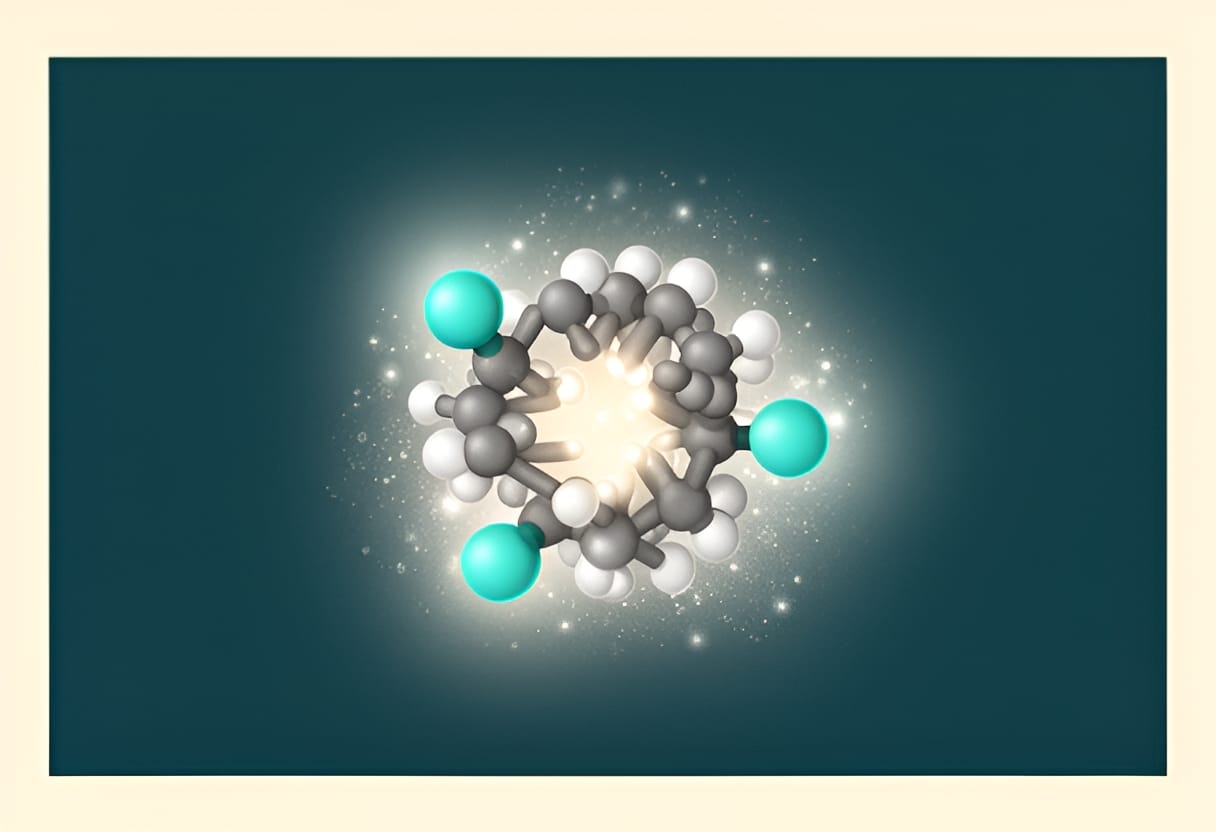
For example, paclitaxel, a highly lipophilic anticancer agent with an intrinsic solubility of less than 0.001 mg/mL, is formulated clinically using Cremophor EL (a nonionic surfactant) at concentrations well above its CMC (~0.02–0.03 mM). In this formulation, paclitaxel is solubilized within the micellar core, enabling intravenous administration. Studies have shown that the apparent solubility of paclitaxel increases by several thousand-fold in the presence of Cremophor EL due to efficient encapsulation in the micellar hydrophobic interior.
Hydrophilic-Lipophilic Balance (HLB) and Surfactant Selection
The hydrophilic-lipophilic balance (HLB) is a quantitative measure of the relative hydrophilicity and lipophilicity of a surfactant, scaled from 0 to 20. Developed by Griffin, the HLB system aids in predicting surfactant behavior and selecting appropriate agents for specific pharmaceutical applications. Low HLB values (3–6) indicate surfactants with strong lipophilic character, suitable for water-in-oil (W/O) emulsions. High HLB values (8–18) reflect greater hydrophilicity, making these surfactants effective for oil-in-water (O/W) emulsions, solubilization, and detergency.
For micellar solubilization of poorly water-soluble drugs, surfactants with HLB values in the range of 13–18 are typically preferred. These surfactants possess sufficient hydrophilicity to remain stably dispersed in aqueous media while providing a hydrophobic core capable of accommodating drug molecules. The optimal HLB for a given drug depends on its molecular structure and lipophilicity; highly lipophilic compounds may require surfactants with HLB values toward the upper end of this range to ensure adequate core hydrophobicity.
Consider the antifungal drug itraconazole, which exhibits pH-dependent solubility and poor aqueous dissolution. Formulation studies have demonstrated that polysorbate 80 (Tween 80), with an HLB of 15, effectively solubilizes itraconazole in aqueous solution. At concentrations above its CMC (approximately 0.01 mM), Tween 80 forms micelles that encapsulate itraconazole molecules, increasing its apparent solubility by over 100-fold. In contrast, surfactants with lower HLB values, such as span 80 (HLB 4.3), fail to form stable micelles in water and instead promote phase separation or oily dispersions, rendering them unsuitable for aqueous solubilization applications.
Surfactant Types in Pharmaceutical Formulations
Pharmaceutical surfactants are broadly classified into ionic (anionic and cationic) and nonionic categories based on the charge of their hydrophilic head group. Each class exhibits distinct properties influencing toxicity, compatibility, and solubilization efficiency.
Nonionic surfactants, such as polysorbates (Tween series), poloxamers (e.g., Pluronic F68, F127), and Solutol HS15, are widely preferred in drug formulations due to their low toxicity, minimal irritation potential, and stability across a broad pH range. They do not ionize in solution, reducing the risk of electrostatic interactions with drug molecules or biological membranes. Their solubilization capacity often increases with temperature, particularly for polyoxyethylene-based surfactants, as thermal energy enhances molecular mobility and micelle dynamics.
Anionic surfactants, including sodium lauryl sulfate (SLS) and sodium dioctyl sulfosuccinate (DOSS), possess negatively charged head groups. While effective solubilizing agents, they may cause mucosal irritation, exhibit incompatibility with cationic excipients or drugs, and are prone to inactivation in the presence of multivalent cations (e.g., Ca²⁺, Mg²⁺) through precipitation. Cationic surfactants, such as benzalkonium chloride and cetyltrimethylammonium bromide (CTAB), carry a positive charge and are associated with higher toxicity and hemolytic activity, limiting their use in parenteral and oral formulations. They are primarily reserved for topical antimicrobial applications where their biocidal properties are advantageous.
The following table summarizes key characteristics of surfactant classes used in pharmaceutics:
| Surfactant Type | Examples | HLB Range | Advantages | Limitations |
|---|---|---|---|---|
| Nonionic | Tween 80, Solutol HS15, Pluronic F127 | 12–18 | Low toxicity, pH stability, minimal ionic interference | Temperature-dependent cloud point, potential oxidation |
| Anionic | Sodium lauryl sulfate, DOSS | 35–40 (effective HLB) | Strong solubilization, good wetting | Irritation, cation sensitivity, incompatibility with cations |
| Cationic | Benzalkonium chloride, CTAB | 13–15 | Antimicrobial properties | High toxicity, hemolysis, incompatibility with anions |
For instance, in the formulation of oral amorphous solid dispersions, polysorbate 80 is frequently employed as a surfactant stabilizer due to its nonionic nature and ability to inhibit crystallization by adsorbing to drug-polymer surfaces. Its HLB of 15 supports effective micelle formation in aqueous gastrointestinal fluids, contributing to enhanced drug dissolution. Conversely, sodium lauryl sulfate, despite its high solubilizing power, is often avoided in soft gelatin capsules due to its tendency to cross-link with gelatin under acidic conditions, potentially compromising shell integrity.
Limitations and Practical Considerations
While micellar solubilization offers a powerful approach to enhancing drug solubility, several limitations must be addressed during formulation development. One significant concern is the potential for mucosal irritation, particularly with ionic surfactants. Sodium lauryl sulfate, for example, has been shown to disrupt lipid membranes in epithelial cells, leading to transient increases in permeability that may be accompanied by discomfort or inflammation. Although nonionic surfactants are generally better tolerated, high concentrations can still provoke local irritation, especially in sensitive populations such as pediatric or geriatric patients.
Another limitation arises from the dilution-dependent nature of micellar systems. Upon administration, especially via oral or intravenous routes, the formulation undergoes rapid dilution in biological fluids. This reduces the surfactant concentration, potentially driving it below the CMC and causing micelle disintegration. If the drug is not absorbed quickly enough, precipitation may occur as the solubilizing capacity diminishes. This phenomenon is particularly relevant for drugs with high dose numbers or slow absorption rates. For example, formulations of danazol using high concentrations of polysorbate 80 have demonstrated precipitation upon dilution in simulated intestinal fluid, underscoring the need to balance surfactant concentration with expected in vivo dilution.
Furthermore, surfactants can interact with other formulation components or biological membranes in ways that impede drug absorption. Polysorbate 80, while generally safe, has been reported to inhibit P-glycoprotein efflux transporters in intestinal cells, which may alter the pharmacokinetics of co-administered drugs. Conversely, some surfactants may sequester drugs too tightly within the micellar core, reducing the free drug concentration available for transcellular permeation—a scenario that can paradoxically decrease bioavailability despite high apparent solubility.
To mitigate these risks, formulation scientists employ strategies such as optimizing surfactant type and concentration to remain just above the CMC, combining surfactants with permeability enhancers or precipitation inhibitors, and selecting nonionic alternatives with favorable safety profiles. For instance, replacing Cremophor EL with polysorbate 80 in paclitaxel formulations has been explored to reduce hypersensitivity reactions, although clinical efficacy and safety must be rigorously evaluated.
In summary, micellar solubilization leverages the self-assembling properties of surfactants to solubilize lipophilic drugs in a hydrophobic microenvironment. Success depends on exceeding the CMC, selecting surfactants with appropriate HLB values for the drug’s lipophilicity, and favoring nonionic agents for reduced toxicity. However, the translational potential of micellar systems is constrained by irritation risks, dilution-induced instability, and interactions with biological systems. Addressing these factors through careful surfactant selection, concentration optimization, and pre-formulation screening is essential for developing safe and effective solubilized formulations.
Cyclodextrins and Inclusion Complexation
Cyclodextrins are cyclic oligosaccharides composed of glucose units linked by α-1,4-glycosidic bonds, forming a toroidal structure with a hydrophobic central cavity and a hydrophilic exterior. This unique architecture enables them to encapsulate poorly water-soluble drug molecules within their cavity through non-covalent interactions, primarily hydrophobic forces, van der Waals forces, and hydrogen bonding. The resulting inclusion complex increases the apparent solubility of the drug by shielding its hydrophobic moieties from the aqueous environment while exposing the hydrophilic cyclodextrin exterior to water.
Among the naturally occurring cyclodextrins, α-, β-, and γ-cyclodextrin differ in the number of glucose units (6, 7, and 8, respectively), which dictates the size of their hydrophobic cavities. β-Cyclodextrin, with a cavity diameter of approximately 6.0–6.5 Å, is the most widely used in pharmaceutical formulations due to its optimal fit for many common drug molecules, such as non-steroidal anti-inflammatory drugs, hormones, and aromatic compounds. Its cavity size allows for effective inclusion of moieties like phenyl rings or alkyl chains, which are frequently present in drug structures. In contrast, α-cyclodextrin’s smaller cavity (4.7–5.2 Å) limits its utility to smaller guests, while γ-cyclodextrin’s larger cavity (7.5–8.3 Å) accommodates larger or multiple guest molecules but is less commonly used due to higher cost and lower complexation efficiency for typical drug sizes.
The strength of the inclusion complex is quantified by the stability constant (K_s), which represents the equilibrium between free drug, free cyclodextrin, and the complex. A higher K_s indicates a stronger association and greater potential for solubilization. Stability constants are typically determined from phase-solubility studies, where the slope of the plot of drug concentration versus cyclodextrin concentration yields the complexation efficiency (CE). A linear plot (A<sub>L</sub> type) with a slope less than 1 suggests 1:1 stoichiometry, while a slope greater than 1 may indicate higher-order complexes or aggregation. The CE, defined as the initial slope of the phase-solubility diagram, reflects the practical utility of the cyclodextrin: a higher CE means more drug is solubilized per unit increase in cyclodextrin concentration.
For example, consider the inclusion complex between ibuprofen and β-cyclodextrin. Phase-solubility analysis reveals an A<sub>L</sub> type profile with a slope of 0.45, indicating a CE of 0.45 and a stability constant (K_s) of approximately 200 M<sup>−1</sup>. This means that for every millimolar increase in β-cyclodextrin concentration, the apparent solubility of ibuprofen increases by 0.45 millimolar. In practical terms, a formulation containing 10 mM β-cyclodextrin can increase the apparent solubility of ibuprofen from its intrinsic solubility of about 0.02 mg/mL to over 0.5 mg/mL, significantly enhancing its dissolution potential.
To address limitations of native β-cyclodextrin, such as its relatively high nephrotoxicity at elevated doses due to slow renal excretion, derivatized cyclodextrins have been developed. Hydroxypropyl-β-cyclodextrin (HP-β-CD) is one of the most widely used modified cyclodextrins in parenteral and oral formulations. The addition of hydroxypropyl groups increases water solubility and reduces the tendency for crystalline aggregate formation, thereby lowering nephrotoxic potential. HP-β-CD retains the ability to form inclusion complexes while exhibiting improved safety and biocompatibility. For instance, HP-β-CD is used in the intravenous formulation of prostaglandin E<sub>1</sub> (alprostadil), where it increases the drug’s aqueous solubility from less than 0.01 mg/mL to over 5 mg/mL, enabling clinical administration.
Despite their utility, cyclodextrin-based formulations face several constraints. The cost of cyclodextrins, particularly modified derivatives, remains higher than many conventional excipients, which can impact large-scale manufacturing. Additionally, while native β-cyclodextrin shows low toxicity at therapeutic doses, chronic or high-dose exposure raises safety concerns, necessitating careful toxicological evaluation. Another limitation is the potential for complex dissociation upon dilution in vivo, which may lead to drug precipitation if the free drug concentration exceeds its intrinsic solubility and absorption is not rapid enough. This is particularly relevant for high-dose drugs where the cyclodextrin concentration required for solubilization may be impractically large.
Nevertheless, cyclodextrins offer a versatile and elegant approach to solubility enhancement that avoids the use of harsh organic solvents or high surfactant concentrations. Their ability to form non-covalent, reversible complexes makes them suitable for a range of dosage forms, including tablets, capsules, topical preparations, and injectables. When combined with other strategies—such as particle size reduction or pH adjustment—cyclodextrin inclusion can contribute to robust formulations that maintain drug stability and improve bioavailability.
Illustration
Molecular structure of β-cyclodextrin showing a toroidal ring of seven glucose units with a hydrophobic interior cavity lined by C–H bonds and a hydrophilic exterior adorned with hydroxyl groups. A drug molecule (e.g., ibuprofen) is depicted partially inserted into the cavity, with its hydrophobic phenyl ring engaged in van der Waals interactions with the cavity wall, while its carboxylic acid group remains exposed to the aqueous environment.
Try This
This week, explore the practical application of cyclodextrins in solubility enhancement through the following steps:
- Retrieve the phase-solubility data for a poorly water-soluble drug (e.g., carbamazepine or fenofibrate) with β-cyclodextrin from a scientific database or literature.
- Plot the apparent drug concentration against cyclodextrin concentration and determine the type of phase-solubility curve (A<sub>L</sub>, A<sub>PS</sub>, or B<sub>s</sub>).
- Calculate the complexation efficiency (CE) from the slope of the linear region and discuss what it implies about the formulation potential.
Key Takeaways
- Cyclodextrins enhance drug solubility by forming inclusion complexes that encapsulate hydrophobic drug moieties within their hydrophobic cavity while maintaining a hydrophilic exterior.
- β-Cyclodextrin is the most commonly used natural cyclodextrin due to its cavity size (6.0–6.5 Å), which complements many drug molecules; modified derivatives like HP-β-CD improve safety and solubility.
- The stability constant (K_s) and complexation efficiency (CE) from phase-solubility studies quantify complex strength and practical utility, guiding formulation decisions.
- Despite limitations such as cost, potential toxicity, and dilution-dependent dissociation, cyclodextrins offer a versatile, non-chemical modification strategy applicable across multiple dosage forms.
- Successful solubilization strategies require matching the approach to the drug’s physicochemical properties, anticipated route of administration, and in vivo behavior to ensure both solubility enhancement and sustained bioavailability.
The molecular recognition between cyclodextrins and guest molecules is governed by a delicate balance of size, polarity, and thermodynamic compatibility. For effective inclusion, the drug molecule—or a significant hydrophobic portion of it—must fit snugly within the cyclodextrin cavity without excessive strain. A guest that is too small may rattle loosely, reducing van der Waals contacts and lowering the stability constant, while one that is too large may only partially insert or induce cyclodextrin distortion, which can destabilize the complex. Polarity also plays a critical role: highly polar or charged groups tend to remain outside the cavity, interacting with the hydrophilic rim or solvent, whereas nonpolar moieties such as aromatic rings, alkyl chains, or steroid cores are driven into the cavity to escape the aqueous environment.
Temperature influences complexation in nuanced ways. While increased thermal energy can enhance molecular motion and collision frequency, it also weakens the relatively weak non-covalent forces that stabilize the inclusion complex. As a result, stability constants often decrease with rising temperature, reflecting the exothermic nature of the inclusion process. This temperature dependence has practical implications for formulation storage and processing; for instance, a complex that is stable at room temperature may partially dissociate under elevated conditions during drying or sterilization, potentially affecting drug release kinetics or physical stability.
A compelling illustration of these principles appears in the formulation of itraconazole, a highly lipophilic antifungal with intrinsic solubility below 0.01 mg/mL. Itraconazole contains a flexible hydrophobic tail and a rigid triazole-containing core. When complexed with hydroxypropyl-β-cyclodextrin (HP-β-CD), the triazole ring and portions of the hydrophobic side chain insert into the cyclodextrin cavity, driven by hydrophobic interactions. Phase-solubility studies reveal an A<sub>L</sub> type profile with a CE of 0.62 and a K<sub>s</sub> of approximately 450 M<sup>−1</sup>, indicating a favorable 1:1 complex. In a solid dispersion prepared by co-evaporation, the apparent solubility of itraconazole increases from less than 0.01 mg/mL to over 0.8 mg/mL in aqueous buffer at pH 6.5. This enhancement supports improved dissolution in simulated intestinal fluid, translating to better pharmacokinetic performance in preclinical models. Notably, the use of HP-β-CD mitigates the nephrotoxicity concerns associated with native β-cyclodextrin, allowing for higher administered doses in oral formulations.
Further optimization can be achieved by considering the stoichiometry of complexation. While 1:1 inclusion is most common, certain elongated or planar drug molecules may form 2:1 (drug:cyclodextrin) or sandwich-like complexes, particularly with γ-cyclodextrin or modified derivatives. For example, flat aromatic systems like porphyrins or certain anthracyclines can simultaneously engage two cyclodextrin molecules—one above and one below the molecular plane—thereby increasing overall complex stability. These higher-order stoichiometries are often detectable through deviation from linearity in phase-solubility plots (yielding A<sub>PS</sub> or B<sub>s</sub> types) or through job plots and spectroscopic titration methods.
In practical formulation development, cyclodextrin complexation is frequently combined with other techniques to maximize benefit. Spray-drying or lyophilization of drug-cyclodextrin mixtures can yield amorphous molecular dispersions where the drug is uniformly distributed at a molecular level, reducing the tendency for crystallization and maintaining the solubilized state. Similarly, incorporating cyclodextrin complexes into matrices such as hydrogels or microspheres allows for controlled release while preserving the solubility advantage. For topical applications, cyclodextrins can enhance the penetration of hydrophobic actives by increasing their thermodynamic activity in the vehicle without causing skin irritation, a significant advantage over surfactant- or co-solvent-based systems.
Ultimately, the success of cyclodextrin-based solubilization hinges on a thorough understanding of the drug’s molecular structure, the thermodynamic parameters of complexation, and the intended biological environment. By aligning these factors, formulation scientists can leverage this supramolecular approach to transform poorly soluble candidates into viable therapeutics.